Using Y DNA to Predict Ancestry: A Statistical Model

Estimating Generational Distance to a Common Ancestor - An Analytical Framework

Copyright 2021 by Barry Teichroeb. All rights reserved.

Introduction

Numerous academic papers have been written and many mathematical models have been built to predict the common ancestor of a comparison set of Y DNA haplotypes. Many times, these have been aimed at determining the most recent common ancestor of a large population and are not necessarily well suited to the analysis of small numbers of samples. Often the mathematical theory underpinning these works is complex and beyond the grasp of non-specialists. Further, the results produced by various approaches can rarely be reconciled. As for the results produced, the interpretation is difficult because the context of the result is often absent. This paper outlines a simpler way to examine a set of haplotypes to arrive at conclusions about the generational distance of the test subjects with richer context as to possible ranges of outcomes and their likelihood. This methodology is suited for application to smaller sample sizes such as those a genealogist would typically work with.

Y DNA is a popular tool for estimating relationships between male descendants for several reasons. There is standardization in testing approaches and test results are easy to work with. An inexpensive 37-marker test is sufficient for reasonably accurate predictions. The markers themselves are stable and mutation rates are low. Many studies have been conducted and provide a large database of mutation rates to use for statistical analysis.

Y DNA possesses an important property for statistical analysis. Any given marker mutates randomly and independently from one generation to the next, and independently from any other marker. As such the value of the markers in a haplotype measured from one generation to the next can be thought of as a Bernoulli process where there are only two possible outcomes: either there is a marker mutation or there is not. Every generational outcome is independent of the others, and the probability of a mutation is constant over the generations.

A Bernoulli process is described mathematically by the binomial distribution, the properties of which enable rich statistical analysis.

Overview of the Binomial Distribution in Terms of Y DNA Mutations

The general form of the binomial formula is:

P[M=m] = (g!/(m! (g-m)!))*r^m*(1-r)^(g-m) where

M = the probability of “m” mutations when

g = the number of generations being considered

r = the mutation rate of the haplotype

For example, suppose the mutation rate for a 37-marker haplotype is 0.191, or about 1 mutation every 5 generations. If we consider the probability of 3 mutations over the course of 8 generations, the binomial formula provides:

m = 3

r = 0.191

g = 8

P[M=1] = (8!/(3!(8-3)!))0.191^3(1-0.191)^(8-3) = 0.136

In this example the probability of 3 mutations in 8 generations is 13.6%.

The probability of 4 mutations in 8 generations is 4%, of 5 mutations is 0.7% and the probability of 3 or more mutations is 18.3%. Using this basic approach, we can build an analytical framework.

Establishing an Analytical Framework

We can describe the probability of equal or greater than m mutations within g generations. This gives us a sense of statistical confidence in any prediction we wish to make. For example, if we observe 3 mutations in a comparison of haplotypes, we can use the binomial formula to tell us that the probability of at least 3 mutations in 13 generations, assuming a mutation rate of 0.191, is about 50%. The probability of at least 3 mutations in 21 generations is 80%.

In this example the term generations means the number of generational transitions creating mutation opportunities. For example, there are 4 transitions between a pair of cousins.

A graph of the probability distribution for 3 mutations looks like this:

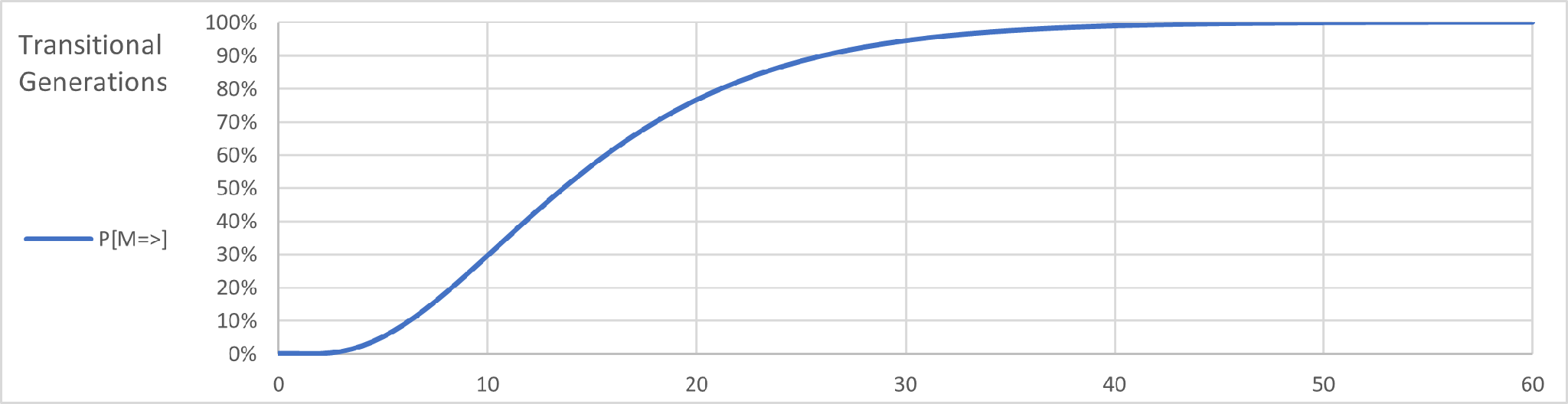
The X-axis show the number of transitional generations for 3 or more mutations and the Y-axis shows the probability of this event. As the number of generations rises it is apparent that the probability of at least 3 mutations becomes closer to 100%.

For genealogical purposes this helps us understand a comparison of Y-DNA tests. Continuing with the same example, if we have two test subjects and their results show 3 mutations, we can conclude that the generational distance between them is about 20 at a probability level of 75%. On average the two subjects would have a common ancestor 10 generations in the past at a confidence level of 75%.

The generational distance between the subjects is 30 at a confidence level of 95%. This indicates, on average, a common ancestor 15 generations in the past. Here is the problem. To establish greater confidence, it is necessary to stretch the ancestral timeline beyond the ability of available genealogical records to prove a family relationship. We can sharpen our understanding of each confidence level but determining the probability of more mutations embodied in the confidence level than we have in our DNA comparison. In our example this means determining the probability of more than 3 mutations at each transitional generation. The binomial formula is employed again and gives us this graph:

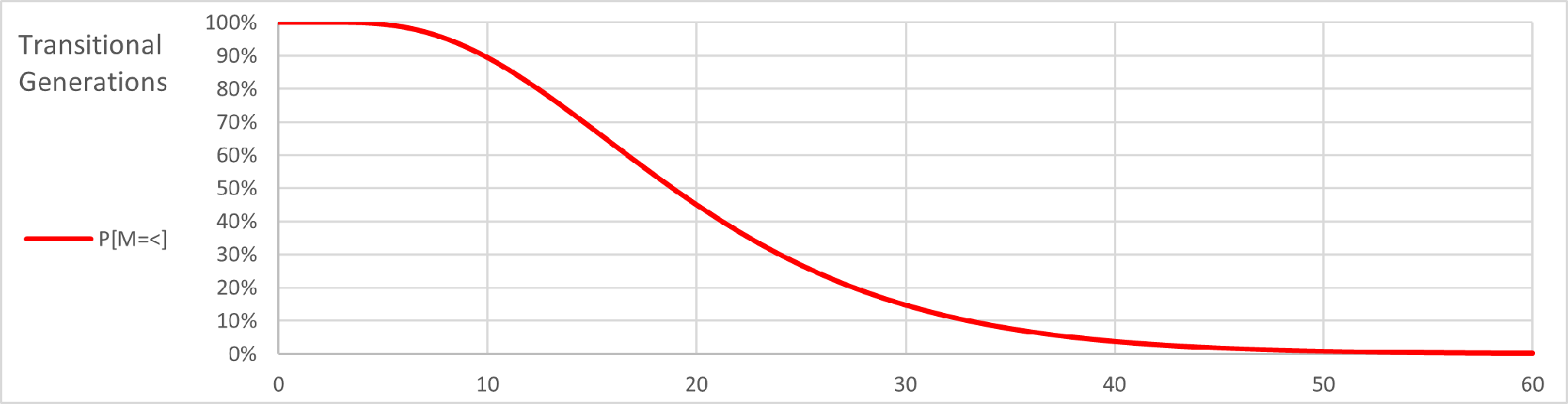
This graph shows the probability of only 3 or fewer mutations at each generational level. If we superimpose the first graph on the second, we have this:

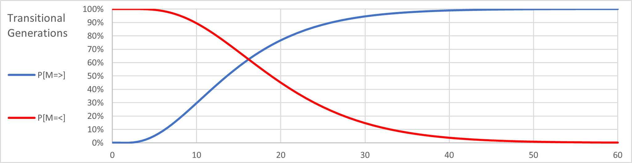
The two plot lines intersect around 16 generations. This means that as the generations increase beyond this point the probability of at least 3 mutations rises but the at the same time the probability of only measuring 3 or fewer mutations falls. For example, at 21 generations we have level of confidence of 80% that at least 3 mutations would occur, but only a 40% probability that at most 3 mutations would occur. By the time we reach the 30 generations needed for a 95% confidence level we see that the probability of only 3 mutations is merely 15%.

I refer to the intersection point as the most likely scenario when assessing the generational distance between test subjects.

Case Study

I am a direct descendant of Michael Teichroeb who was born around 1740. Between us there are 6 generations. In addition to my 37-Marker Y-DNA test there are two other samples. One is also a descendant of Michael. The other is a descendant of Johann Teichroeb who was born in 1744. Coincidently, I am a matrilineal descendant of Johann, and there are 8 generations between us. There are valid genealogical reasons to think Michael and Johann are related. What can the Y-DNA tests tell us about the likelihood these two men were brothers?

In total there were 34 matching markers and 3 mutations in the test results:

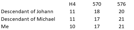
I do not know who the other two test subjects are and can only guess that they are roughly at the same generational level as me in relation to Michael and Johann. If Michael and Johann are brothers, then the common ancestor is their father. I am 7 generations removed from this ancestor. If the descendant of Johann is roughly my age, then he must be 8 – 10 generations removed from this common ancestor. I know enough about my own family tree to be certain the other descendant of Michael is no closer in relationship to me than my great-grandfather and therefore at least 3 generations distant; he could be as many as 7 generations distant.

Combining all of this we have a genealogical range of transitional generations of 18 – 24.

Using the probability graph above, it seems likely there are around 16 transitional generations among the three test subjects and the common ancestor. This is at the low end of the genealogical range.

At the 80% confidence level about 21 generations are required to have 3 mutations, and at this point there is only a 40% probability of 3 or fewer mutations. This is at the midpoint of the genealogical range.

If we move up to the 90% confidence level, we need about 25 generations, which is at the high end of the genealogical range. At this point there is only a 25% probability of 3 or fewer mutations.

The statistical evidence in correspondence with the genealogical data available indicates a high level of confidence that Michael and Johann were brothers. As the confidence level increases to a point of great certainty it is accompanied by a strong probability that we would see more than 3 mutations, thus pushing our estimated transitional generations back toward the genealogical range we determined.

Conclusion

A thorough assessment of statistical outcomes requires more than just confidence probabilities to arrive at useful genealogical conclusions. It is not enough to know with high confidence the extreme generational level necessary for the number of mutations observed in a comparison of samples. It is necessary to know the probability that this level of confidence corresponds to more mutations than actually observed. Further, it is apparent that some understanding of the genealogy of the individuals, however hypothetical, is needed to interpret the statistical results.

Appendix – Mutation Rates

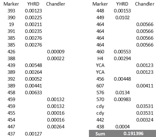
In accordance with Nordtvedt (Nordtvedt 1998) the mutation rate of a haplotype is the sum of the mutation rates of the markers it contains.

The mutation rates used in this paper are a composite of rates from the YHRD database and Chandler rates where YHRD rates are not available. The rates are in the table below.

References

Chandler John F, Estimating Per-Locus Mutation Rates, Journal of Genetic Genealogy 2:27-33, 2006.

Nordtvedt K, More Realistic TRMCA Calculations, Journal of Genetic Genealogy 4(2):96-103, 2008.

Y Chromosome Haplotype Database, https://YHRD.org.